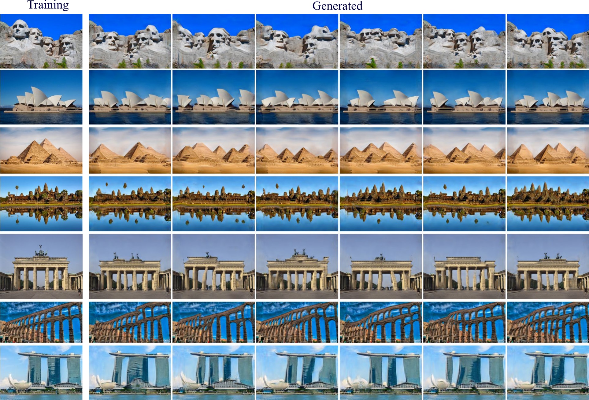
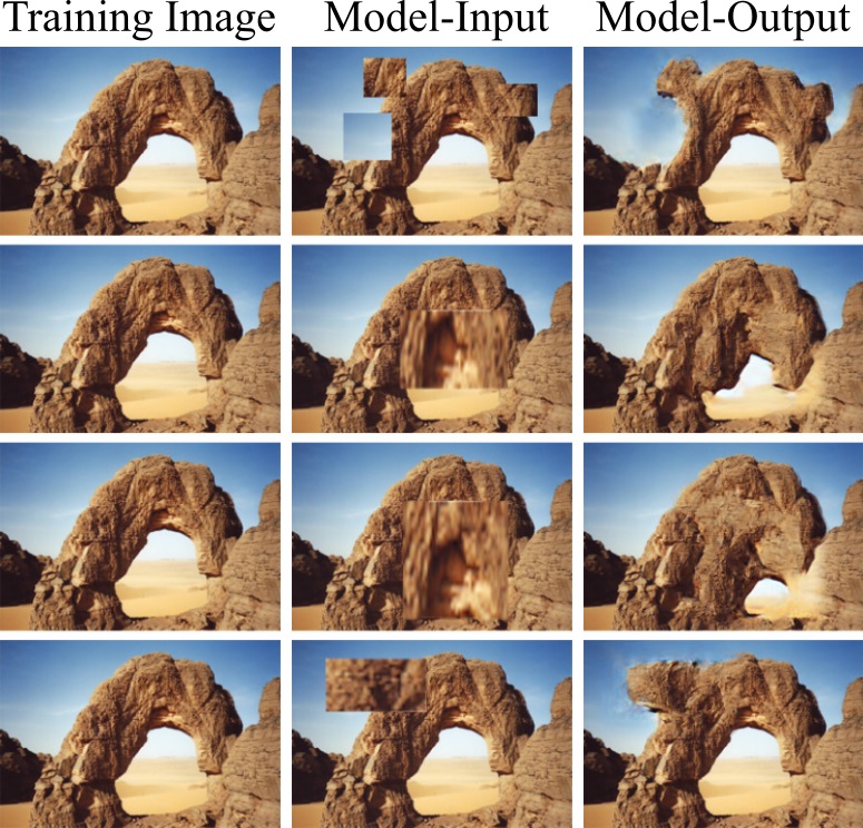
Recently there has been an interest in the potential of learning generative models from a single image, as opposed to from a large dataset. This task is of practical significance, as it means that generative models can be used in domains where collecting a large dataset is not feasible. Fig. 1 shows an example of what a model trained on only a single image can generate.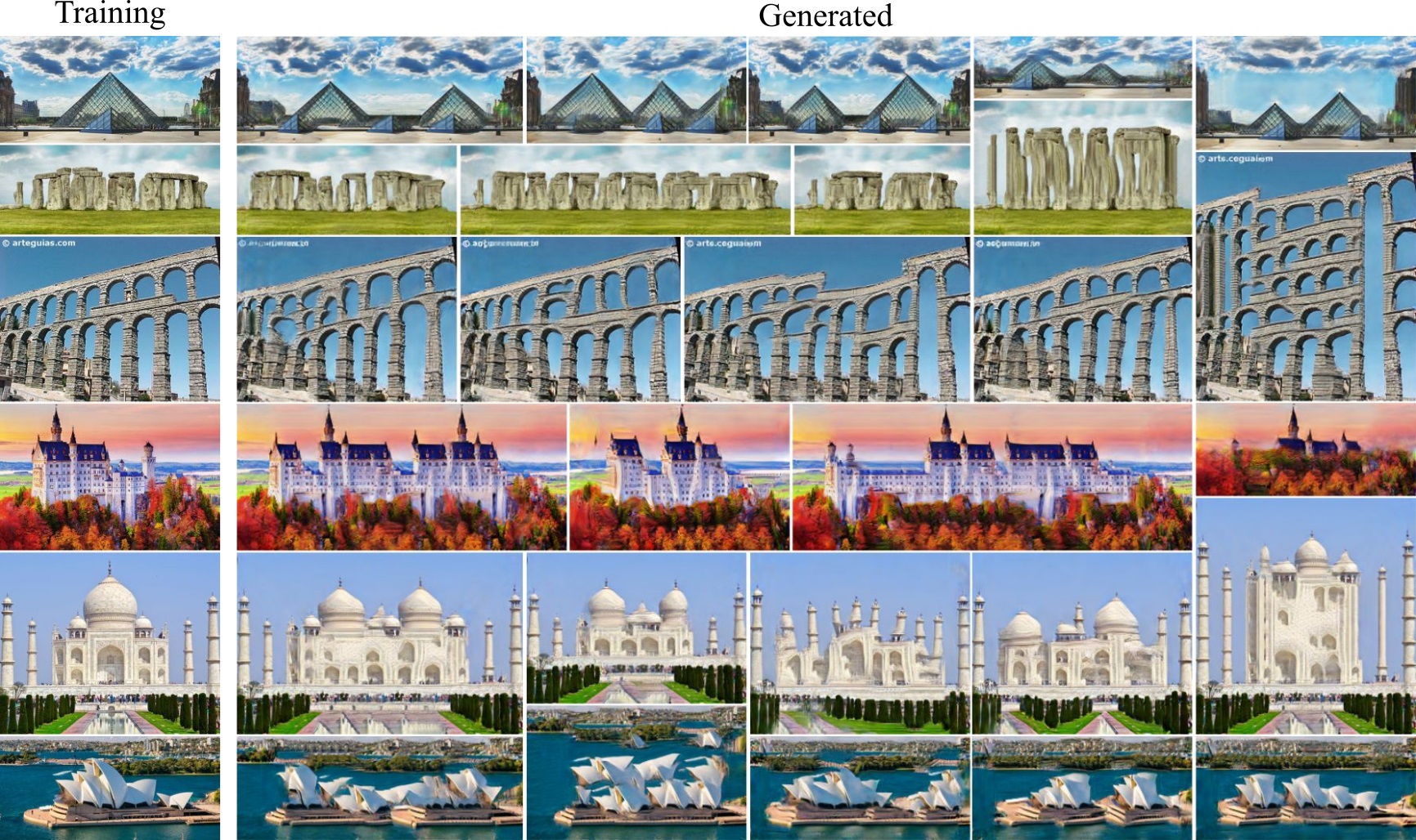

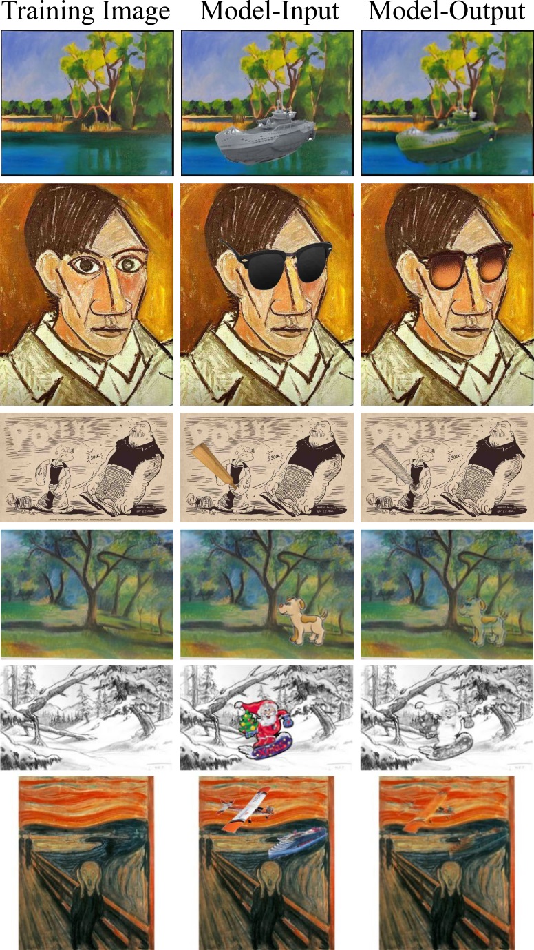
Single-image generative models can also be used for many other tasks such as image super-resolution, image animation, and image dehazing. Fig. 2 and Fig. 3 show some examples of our model applied to image harmonization and image editing.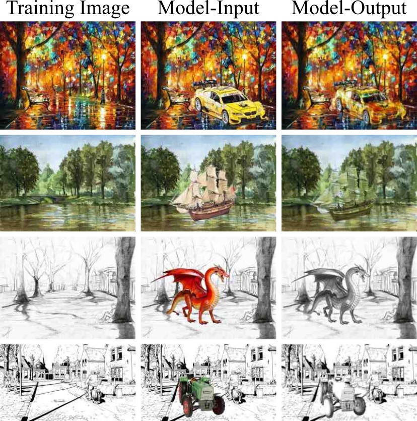

You can even use them for tasks such as image animation as seen in Fig. 4.

The first work that introduced GANs for unconditional image generation trained on a single natural image was SinGAN, presented at ICCV 2019. Before that, several other approaches trained GANs on single images, however, these images where either not natural images (e.g. these approaches for texture synthesis) or the task was not to learn an unconditional model (e.g. InGAN for image retargeting). This blog post summarizes our paper Improved Techniques for Training Single-Image GANs in which we look into several mechanisms that improve the training and generation capabilities of GANs on single images.

Our main contributions, which we will summarize in the following post, are:

• training architecture and optimization: we identify several aspects of the architecture and optimization process that are critical to the success of training Single-Image GANs;
• rescaling approach for multi-stage training on different resolutions: the approach to rescale images for the different training stages directly affects the number of stages we need to train on;
• fine-tuning approach for several tasks: we introduce a fine-tuning step on pre-trained models to obtain even better results on tasks such as image harmonization.

In the following, we will talk about each of these points in a bit more detail, before showing some of our results.

Training Architecture and Optimization

To put our approach into perspective we quickly describe SinGAN’s training procedure, before giving a more detailed overview of our approach. SinGAN trains several individual generator networks on images of increasing resolutions. Here, the first generator - working on the smallest image resolution - is the only unconditional generator that generates a image from random noise (see Fig. 5 for a visualization).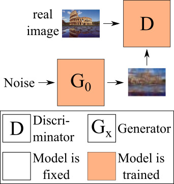

The important part is that the discriminator is a patch discriminator, i.e. the discriminator never sees the image as a whole, but only parts of it. Through this it learns what “real” image patches look like. Since the discriminator never sees the image as a whole the generator can fool it by generating images that are different from the training image on a global perspective, but similar when looking only at patch statistics.

The generators working on higher resolutions take the image generated by the previous generator as input and generate an image of the current (higher) resolution from it. All generators are trained in isolation, meaning all previous generators’ weights are kept frozen when training the current generator. Fig. 6 shows a visualization of how the training proceeds throughout the different resolutions.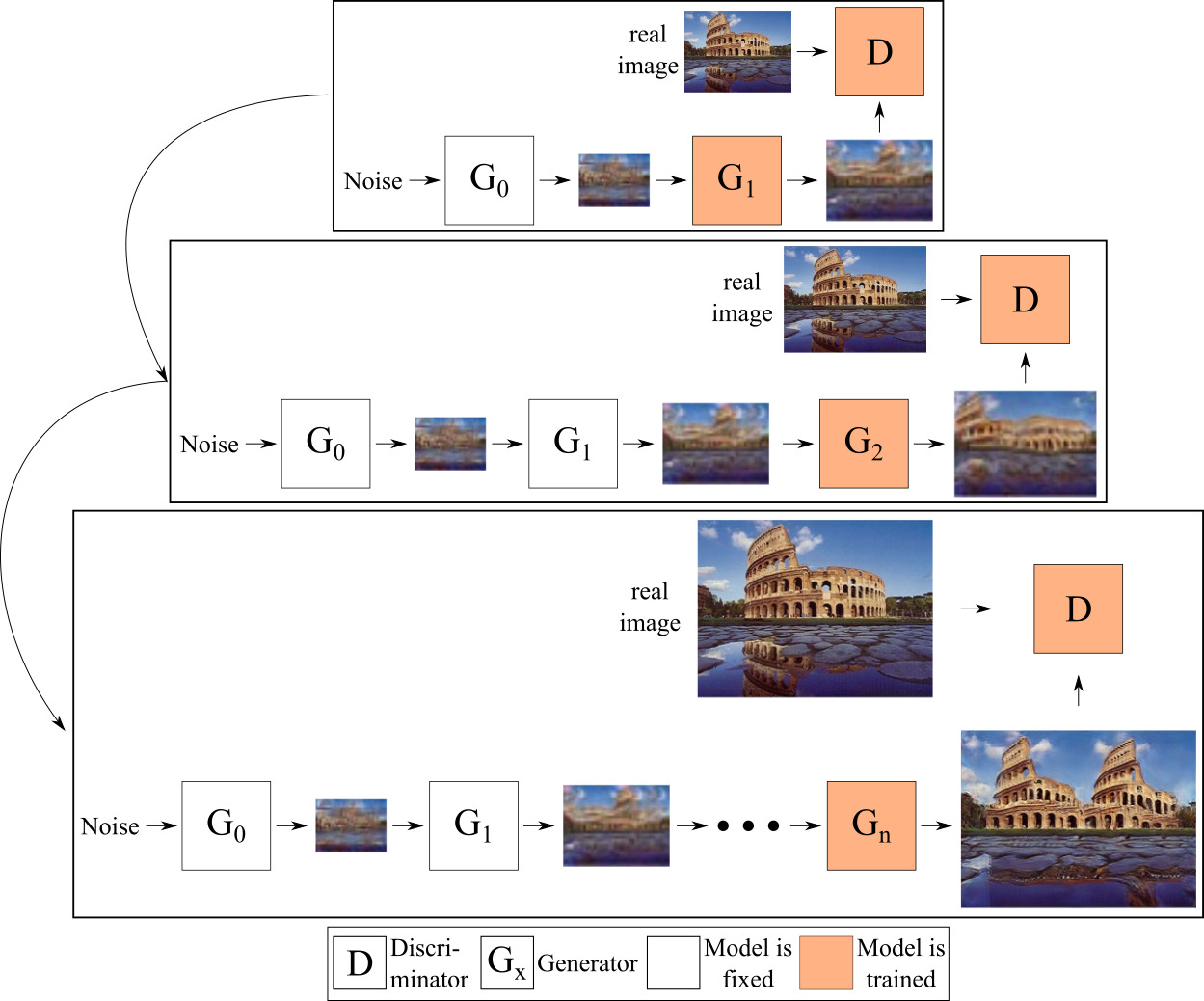

During our experiments we observe that training only one generator at a given time, as well as propagating images instead of feature maps from one generator to the next, limits the interactions between the generators. As a consequence, we train our generators end-to-end, i.e. we train more than one generator at a given time, and each generator takes as input the features (instead of images) generated by the previous generator. Since we train several generators concurrently, we call our model the *Concurrent-Single-Image-GAN” (ConSinGAN). See Fig. 7 for a visualization.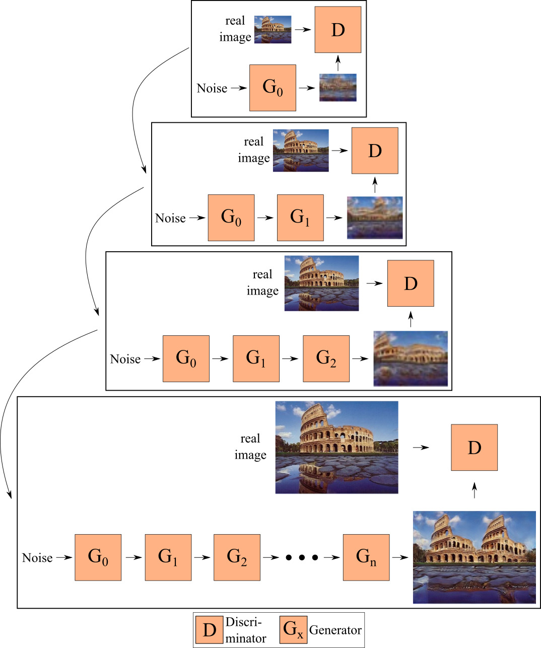

Now, the problem with training all generators is that this quickly leads to overfitting. This means that the final model does not generate any “new” images, but instead only generates the training image, which is obviously not what we want. We introduce two ways of how to prevent this from happening:

1. only train some of the generators at any given time, not all of them and
2. use different learning rates for the different generators, with smaller learning rates for earlier generators when training a given generator.

Fig. 8 visualizes our model with these two approaches implemented. As a default, we train up to three generators concurrently and scale the learning rate by 1/10 and 1/100 respectively for the lower generators.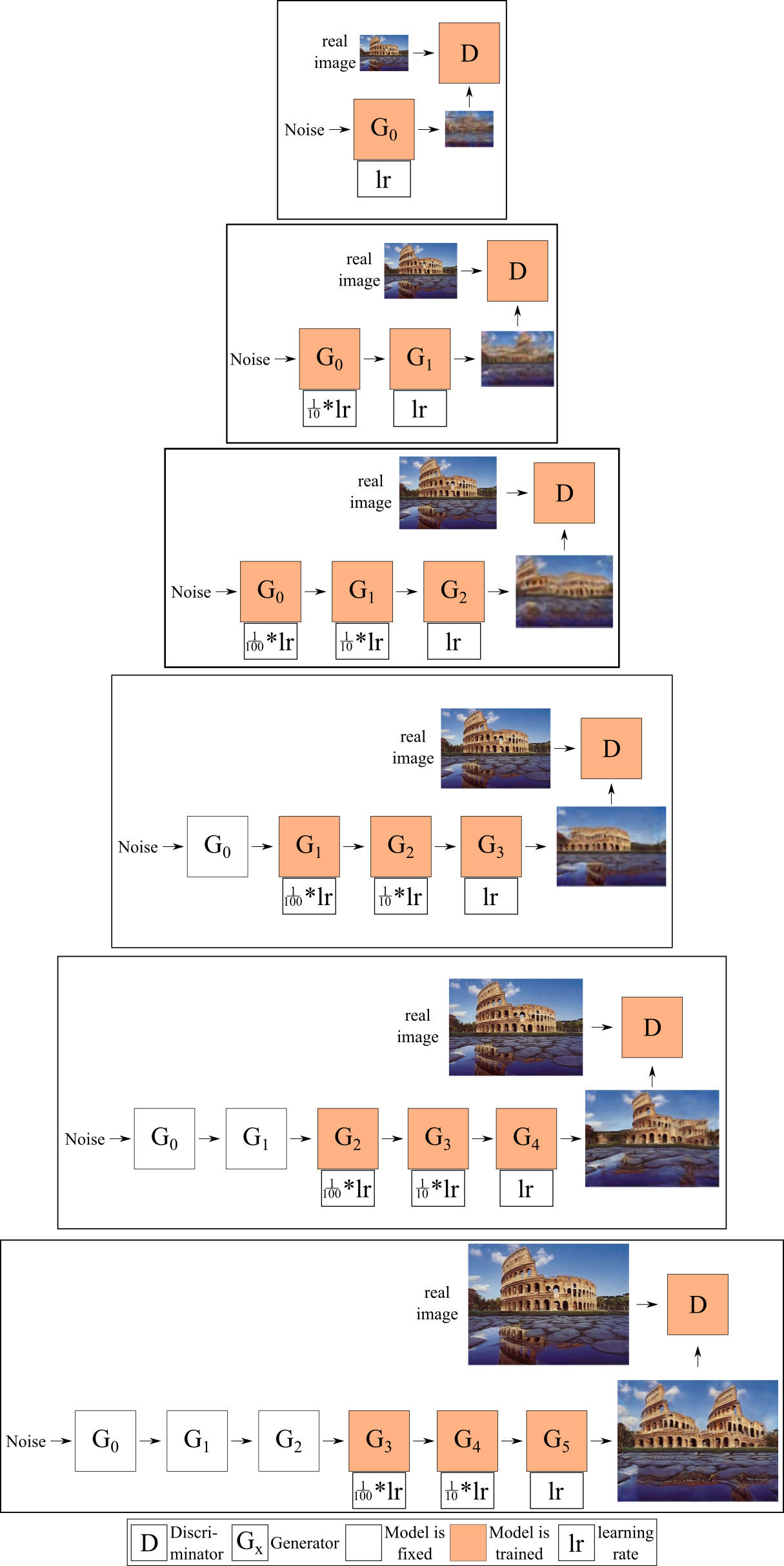

One interesting aspect of this approach is that we are now able to trade-off image diversity for fidelity by changing, e.g., the way of how we scale the learning rate for lower generators. Using a larger learning rate for the lower generators means that the generated images will, on average, be more similar to the training image. Using smaller learning rates for the lower generators, on the other hand, means that we will have more diversity (of possibly worse quality) in the generated images. Fig. 9 shows an example of what this might look like and we can see that larger learning rates of lower generators results in better image fidelity but less image diversity.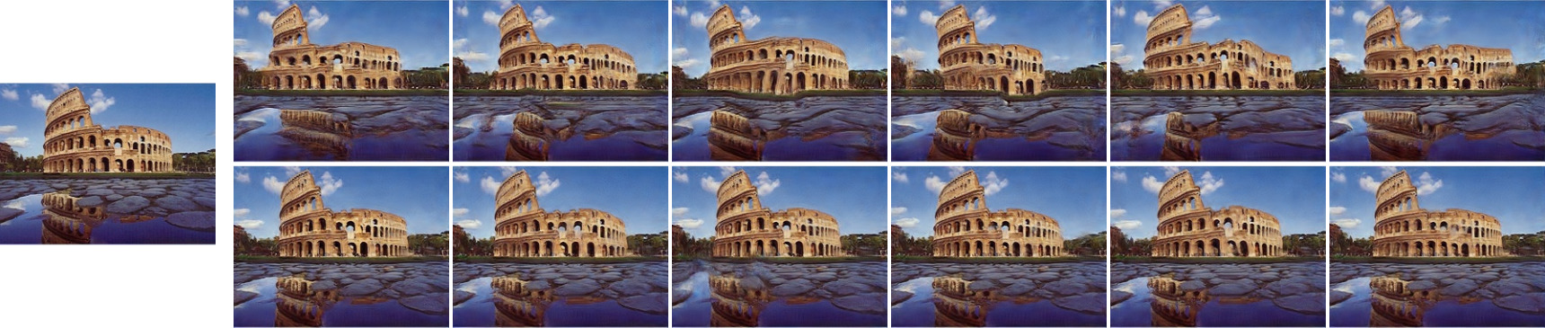

Improved Rescaling

While training the GAN on several stages of different resolutions seems to be a good way of training a GAN on a single image, the question is how many stages we need to train on until we can generate good images. The original SinGAN model, on average, needs to train on 8-10 individual stages. This obviously increases both the number of parameters in the model and the training time.

SinGAN originally rescales images by multiplying the image resolution of the final generator $G_N$ (e.g. 250x250 px) with a scaling factor $r$ for each stage. This means that for a given stage $n$, the image resolution that is used to train it is: \begin{equation} x_n = x_N\times r^{N-n}, \end{equation} where $r=0.75$ is used as default value for the scaling factor and $x_N$ is the image resolution used for the final generator.

We can downsample the images more aggressively to train the model on fewer stages, e.g. by using $r=0.55$. However, if we do this with the original rescaling approach the generated images lose much of their global coherence.

We observe that this is the case when there are not enough stages at low resolution (roughly fewer than 60 pixels at the longer side). Consequently, to achieve image consistency we need a certain number of stages (usually at least three) at low resolution. However, we observe that we do not need many stages a high resolution. Based on this observation we adapt the rescaling to not be strictly geometric (i.e. $x_n = x_N\times r^{N-n}$), but instead to keep the density of low-resolution stages higher than the density of high-resolution stages: \begin{equation} x_n = x_N\times r^{((N-1)/\textit{log}(N))*\textit{log}(N-n)+1}\ \text{for}\ n=0, …, N-1. \end{equation}

For example, for an image $x_N$ of resolution 188x250 px using the new and old rescaling approaches leads to the following resolutions: \begin{aligned} 10&\text{ Stages - Old Rescaling: }\mkern-38mu &&25\times34, 32\times42, 40\times53, 49\times66,\ \ 62\times82, \ \ \ \ 77\times102, 96\times128, 121\times160, 151\times200, 188\times250 \\ 10&\text{ Stages - New Rescaling: }\mkern-38mu &&25\times34, 28\times37, 31\times41, 35\times47,\ \ 41\times54,\ \ \ \ 49\times65,\ \ 62\times82,\ \ \ \ 86\times114, 151\times200, 188\times250 \\ 6&\text{ Stages - Old Rescaling: }\mkern-38mu &&25\times34, 38\times50, 57\times75, 84\times112,126\times167,188\times250 \\ 6&\text{ Stages - New Rescaling: }\mkern-38mu &&25\times34, 32\times42, 42\times56, 63\times84, \ \ 126\times167, 188\times250 \end{aligned}

We can see that, compared to the original rescaling method, we have more stages that are trained on smaller resolutions, but fewer stages that are trained on higher resolutions. Using this approach we can train our model on six stages and still generate images of the same quality as models trained on 10 stages with the old rescaling method.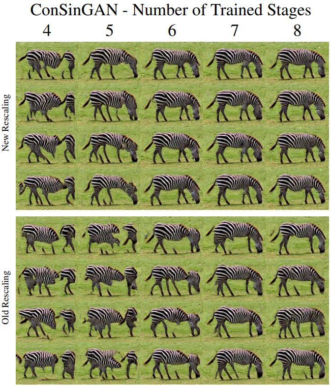

Fine-tuning for Image Harmonization

Finally, since our model can be trained end-to-end we introduce a novel fine-tuning step for tasks such as image harmonization. Image harmonization is the task were you have a given image of a given style (e.g. a painting) and you want to add an object to that image that should adhere to the overall image style. For this, we first train our model on the training image as described previously. Once the model is fully trained we can additionally train it on the given “naive” image to achieve even better results. Fig. 11 shows an example of this.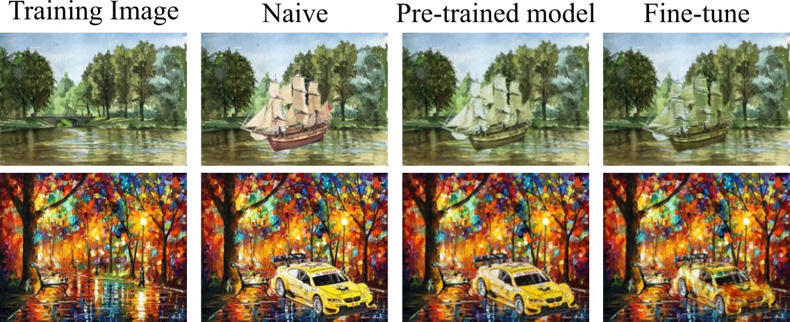

Results

We now show a small sample of our results. For more results, comparisons to SinGAN, and details please refer to our paper and supplementary material or try it for yourself with the code we provide.